Tiny Organoid Segmentation and Coordinate Calculation

Download

The goal of this assay workflow is to detect and analyze one small organoid within an image group of high magnification MCAM images. When imaging a 96-well plate at 10x magnification with the Vireo, it is necessary to scan the well plate, acquiring multiple overlapping images of each well which are stitched together for visualization. Within the image group, we look to detect the organoids of interest in all images and then filter out those on the edges of images. After that, we select the one organoid where the algorithm has the highest confidence, and then analyze this single best organoid with regard to area and circularity. Coordinates of the locations of the organoids can also be exported in a CSV format. The following workflow steps through acquisition, data reduction, and analysis of grouped image datasets for single organoid detection and analysis of tiny organoids.

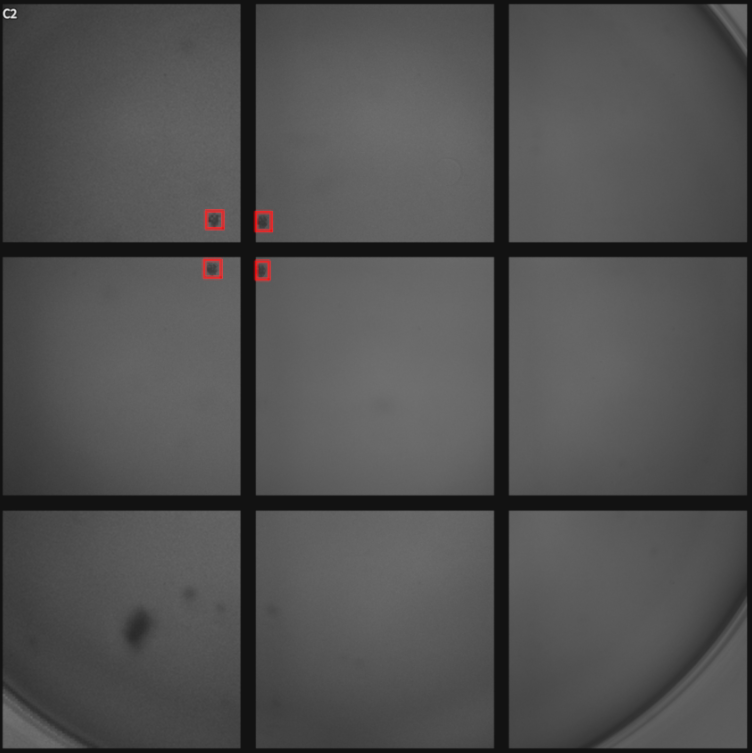
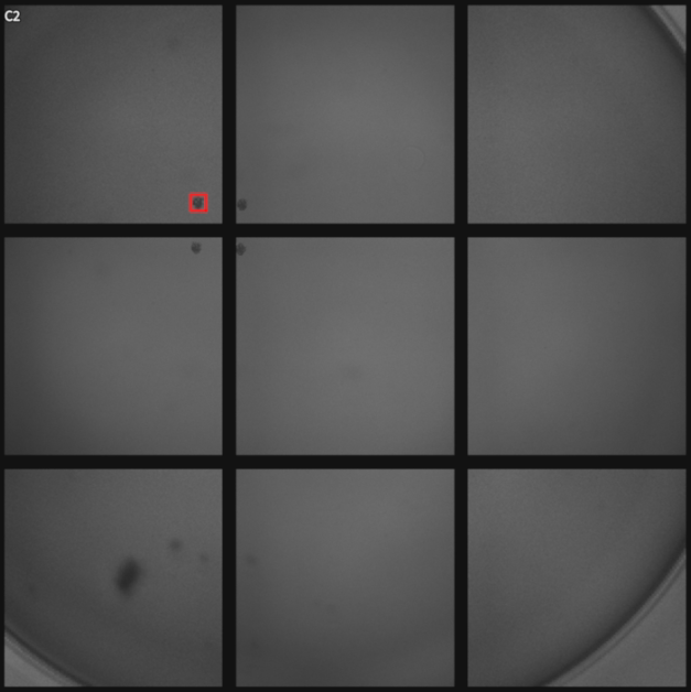
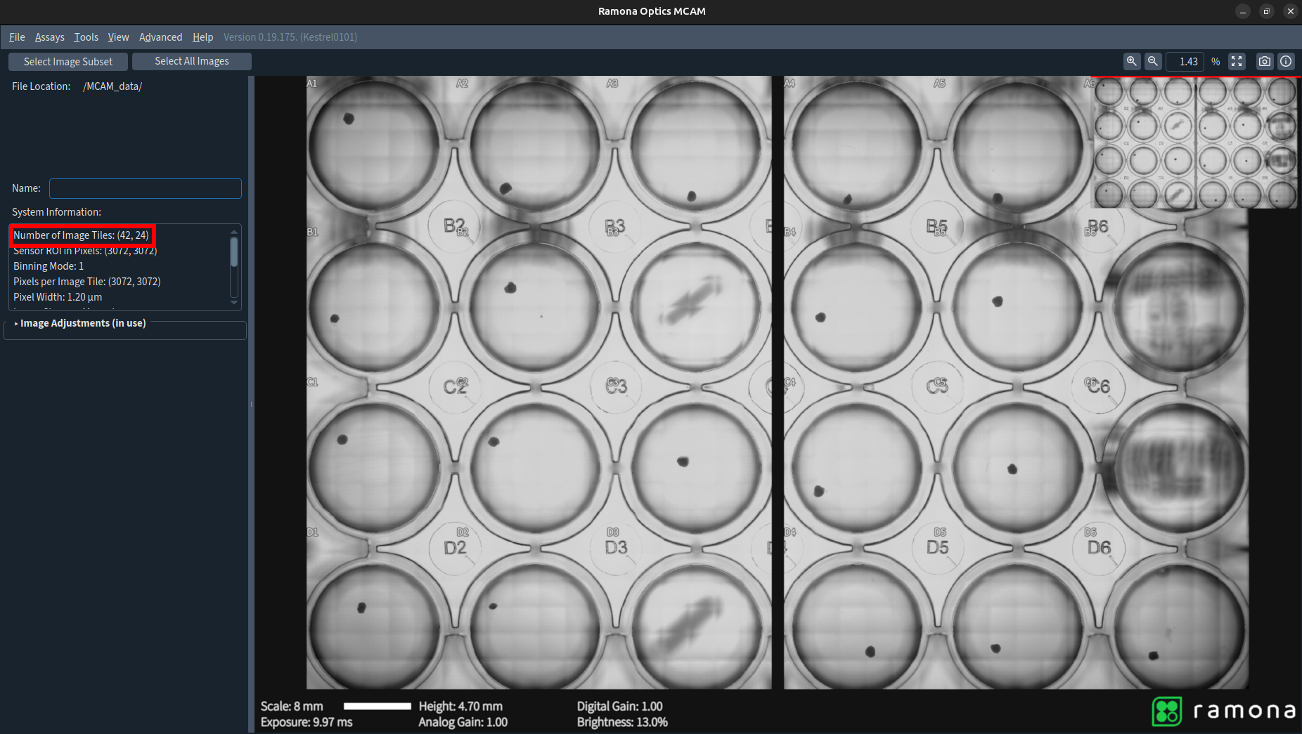
Step	Function
1	Acquire a well plate scan using the 10x 3x3 acquisition mode described in the Workflow Guide SOP “Full Well Scan”.
2	Locate and open your acquired XYZC-stack acquisition dataset in the MCAM Viewer by either double clicking on the metadata.nc file or opening the Viewer software from the left desktop toolbar and drag and drop the metadata.nc file into the Viewer.
3	Project the dataset following the instructions described in the “Stack Projections” workflow protocol selecting the “Tiny Organoid” projection.
4	Once the projection processing has completed, close the MCAM Viewer window, locate and open the newly projected dataset in the MCAM viewer.
5	Go to Assays > Segmentation.
6	Select the “Tiny Single Organoid Focus” model under “Bounding Box Model Selection”. Both filters “Filter Boundary” and “Filter Highest Confidence” are correctly selected by default when using this model. The segmentation model selection does not need to be changed.
7	Click “Select Alignment” under “Output Options”to apply the alignment file (refer to “Create a Well Alignment File” on how to create one). Make sure the box for “Export Bounding Box Coordinates” is checked. Choose the Coordinate Units you’d prefer in the output.
8	Choose Coordinate Units and Area Units.
9	Click “Segment Dataset” to initiate the analysis.
10	Visualization of the segmentation results is overlaid on images in the MCAM Viewer and quantified metric results are exported in .CSV format in the “segmentation_analysis_results” folder located within the focus projection dataset directory.
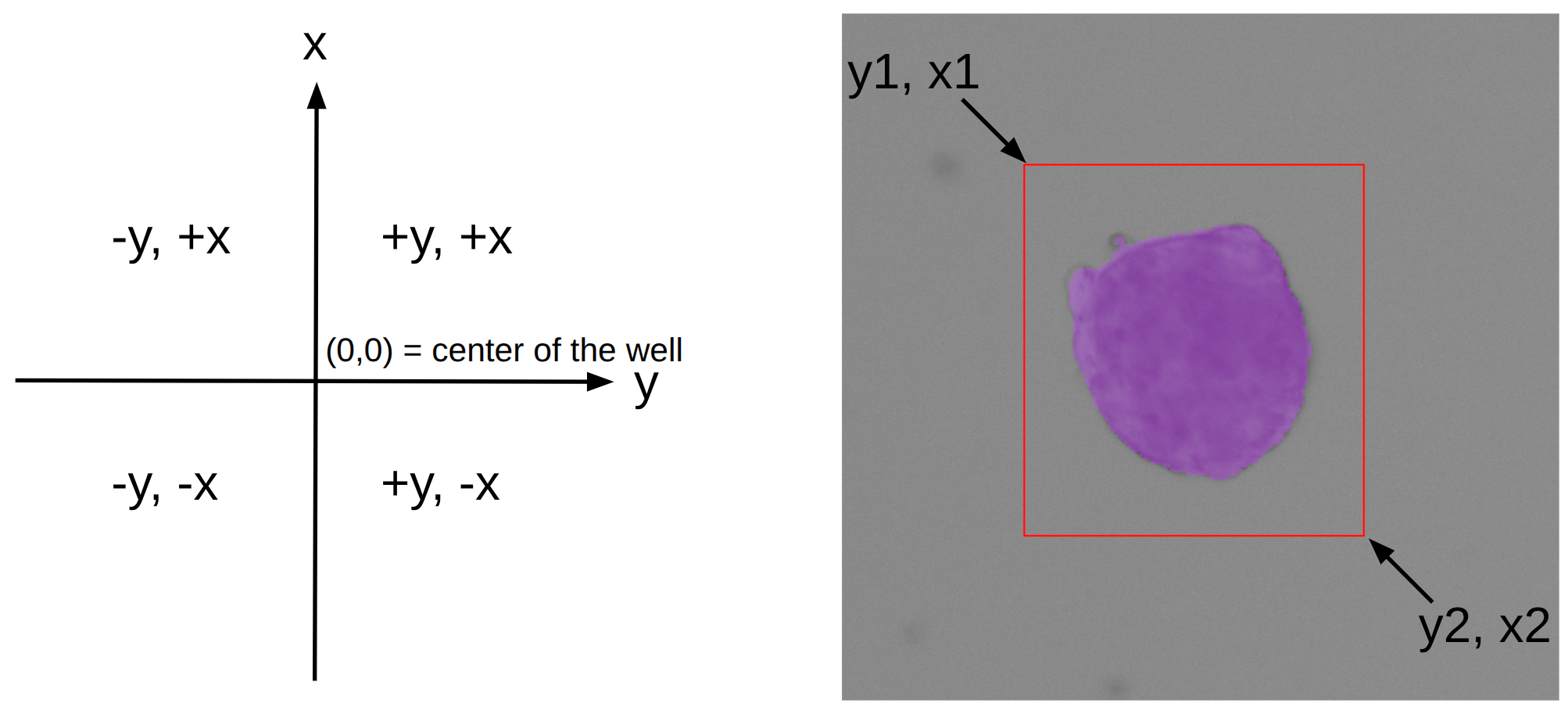
11	Orientation and interpretation: Coordinates are output in 3 ways: the distance from the center of the well to top-left (y1, x1) and bottom-right corners (y2, x2), and center of the bounding box (see figure below for orientation of coordinates and interpretation of the CSV output).

Left: y,x coordinates of the center of the well, with relative locations indicated by plus (+) and minus (-) symbols. Right: Notation indicating the top-left and bottom-right corners of a bounding box.