5. Animal Tracking Data Analysis
Organism tracking is performed through the MCAM GUI resulting in .CSV output files containing tracking data. This page explores concepts relating to loading data from the CSVs, plotting data, and filtering data.
Output Files
Output files are saved in a folder with the same name as the input file and this folder is created in the parent directory of the input file.
Raw Tracking Data - tracking_data.csv - CSV file
containing 8 key-points per fish, x, y coordinate and
confidence for each keypoint. Note: This file is likely
too large to be opened in Excel or other spreadsheet
software due to the large number of columns in the
data array. This file can be opened and manipulated
using Python.
Plotted Tracks -
plotted_tracks.png- Visualization of movement over time from blue (earliest, cold) to red (most recent, hot).Distance Traveled Data -
distance_traveled_metrics.csv- Distance traveled and speed calculated for each frame.Aggregate Metrics -
distance_traveled_key_metrics.csv- Distance traveled and speed calculated for each frame.Video Composite -
composite_tracked_video.mp4- MP4 video containing key-point and skeleton labeled fish for all wells of a well plate.
Units
Unless otherwise specified, exported units implicitly:
Distance or length: meters
Time: seconds
Velocity or speed: meters/second
Orientation/Angle: degrees
Zebrafish Examples
Zebrafish Tracking Workflow
 1"""
 2# %% Sample zebrafish tracking workflow script
 3# By Ramona Optics Inc. Copyright 2023-2025
 4
 5This script provides an example to walk through the steps of the tracking workflow.
 6
 7"""
 8
 9from pathlib import Path
10
11from tqdm import tqdm
12
13from owl import mcam_data
14from owl.analysis.models import fetch_model, zebrafish_models_recommended
15from owl.analysis.tracking import infer_dataset
16from owl.analysis.tracking_data_analysis import (
17    compute_fish_length,
18    export_csv,
19    generate_tracking_dataset,
20    make_dataframe,
21)
22from owl.visualize.tracking import plot_tracks_from_dataset
23
24# %% define the project path where outputs are collected
25exported_path = '/MCAM_data/EXPORTED_FOLDER_YOU_WANT_TO_TRACK'
26
27# %% load the exported dataset video file
28video_dataset = mcam_data.load(exported_path)
29
30# %% determine the well plate configuration, i.e. 24, 48 or 96 well plate
31well_plate = (int(video_dataset.wellplate_config_rows) *
32              int(video_dataset.wellplate_config_columns))
33
34# %% create a results folder within the output data path
35tracking_filepath = Path(exported_path)
36results_folder = tracking_filepath / 'results'
37results_folder.mkdir(parents=True, exist_ok=True)
38
39# %% download and point to a pre-trained tracking model
40recommended_model_name = zebrafish_models_recommended[f"{well_plate}_well_plate"]
41model_path = fetch_model(recommended_model_name)
42
43tracking_dataset = infer_dataset(
44    video_dataset,
45    model_path,
46    tqdm=tqdm,
47)
48
49# %% make computations based on raw tracking data and store them in the dataset
50tracking_dataset['fish_length_information'] = compute_fish_length(tracking_dataset)
51
52# %% plot the tracks on representative images, color gradient represents speed
53plot_tracks_from_dataset(
54    tracking_dataset,
55    output_filename=results_folder / 'plotted_tracks.png',
56    apply_circle_mask=True,
57    apply_square_mask=False,
58    speed=True,
59)
60
61# %% save the tracking data separately from the dataset for future analysis
62# the images are already saved so we do not save them again
63tracking_dataset = tracking_dataset.drop_vars('images')
64tracking_dataset.to_netcdf(tracking_filepath / 'tracking_metadata.nc')
65
66# %% prepare tracking dataset for export to csv format including unit conversions
67tracking_dataset = generate_tracking_dataset(tracking_dataset)
68
69# %% prepare raw tracking data for export
70tracking_output_df, header = make_dataframe(
71    tracking_dataset,
72    information_name='tracking_information',
73    row_index='time',
74    column_indices=('well_row_letter',
75                    'well_column_number',
76                    'tracking_keypoint',
77                    'tracking_location'),
78)
79# %% save the raw tracking data
80export_csv(
81    tracking_output_df,
82    results_folder / 'tracking_data.csv',
83    header=header,
84    index=True
85)
Tracking Dataset - Data Filtering
 1"""
 2# %% Sample zebrafish tracking workflow script
 3# By Ramona Optics Inc. Copyright 2023-2025
 4
 5This script provides an example to filter tracking data using
 6anomaly detection and denoising.
 7
 8"""
 9
10from pathlib import Path
11
12from owl.analysis.tracking_data_analysis import (
13    compile_derived_metrics,
14    compute_fish_length,
15    export_csv,
16    filter_anomalies,
17    generate_tracking_dataset,
18    get_anomaly_mask_well_radius,
19    load_tracking_dataset,
20    make_dataframe,
21)
22from owl.visualize.tracking import plot_tracks_from_dataset
23
24# %% define the project path where outputs are collected
25exported_path = '/MCAM_data/EXPORTED_FOLDER_YOU_WANT_TO_TRACK'
26
27# %% create a results folder within the output data path
28tracking_filepath = Path(exported_path)
29results_folder = tracking_filepath / 'results'
30results_folder.mkdir(parents=True, exist_ok=True)
31
32# %% load the previously tracked dataset
33tracking_dataset = load_tracking_dataset(exported_path)
34
35# %% fish length must be computed prior to anomaly detection
36tracking_dataset['fish_length_information'] = compute_fish_length(tracking_dataset)
37
38# %% determine the well plate configuration, i.e. 24, 48 or 96 well plate
39well_plate = (int(tracking_dataset.wellplate_config_rows) *
40              int(tracking_dataset.wellplate_config_columns))
41
42# %% detect anomalous data, remove it and interpolate to replace missing data
43anomaly_mask_well_radius = get_anomaly_mask_well_radius(
44    well_plate, apply_circle_mask=True,
45)
46tracking_dataset['tracking_information'][...], filtering_information = filter_anomalies(
47    tracking_dataset, well_radius=anomaly_mask_well_radius
48)
49tracking_dataset['filtering_information'] = filtering_information
50
51# %% plot the tracks on representative images, color gradient represents speed
52plot_tracks_from_dataset(
53    tracking_dataset,
54    output_filename=results_folder / 'plotted_tracks.png',
55    apply_circle_mask=True,
56    apply_square_mask=False,
57    speed=True,
58)
59
60# %% convert the dataset from pixel coordinates to SI units
61tracking_dataset = generate_tracking_dataset(tracking_dataset)
62
63# %% compute distance traveled and speed metrics with denoising
64tracking_dataset, denoising_information = compile_derived_metrics(
65    tracking_dataset,
66    denoise=True,
67)
68tracking_dataset['denoising_information'] = denoising_information
69
70# %% prepare movement metric data for export
71metrics_output_df, header = make_dataframe(
72    tracking_dataset,
73    information_name='movement_metrics',
74    row_index='time',
75    column_indices=('well_row_letter',
76                    'well_column_number',
77                    'tracking_metrics',),
78)
79
80# %% save the distance traveled data
81export_csv(metrics_output_df,
82           results_folder / 'distance_traveled_metrics.csv',
83           header=header,
84           index=True)
Tracking Dataset - Time Binning
 1"""
 2# %% Sample zebrafish tracking workflow script
 3# By Ramona Optics Inc. Copyright 2023-2025
 4
 5This script is an example to bin tracking data by one second intervals.
 6
 7"""
 8
 9from pathlib import Path
10
11from owl.analysis.tracking_data_analysis import (
12    compile_derived_metrics,
13    export_csv,
14    generate_tracking_dataset,
15    load_tracking_dataset,
16    make_dataframe,
17)
18
19# %% define the project path where outputs are collected
20exported_path = '/MCAM_data/EXPORTED_FOLDER_YOU_WANT_TO_TRACK'
21
22# %% time bin given in seconds
23time_bin = 1
24
25# %% load a previously tracked dataset
26tracking_dataset = load_tracking_dataset(exported_path)
27
28# %% ensure a results folder exists within the output data path
29tracking_filepath = Path(exported_path)
30results_folder = tracking_filepath / 'results'
31results_folder.mkdir(parents=True, exist_ok=True)
32
33# %% prepare tracking dataset for export including unit conversions
34tracking_dataset = generate_tracking_dataset(tracking_dataset)
35
36# %% calculate distance traveled and speed. this function should be
37# run after 'generate_tracking_dataset' to ensure SI units
38tracking_dataset = compile_derived_metrics(tracking_dataset)
39
40# %% prepare movement metric data for export
41metrics_output_df, header = make_dataframe(
42    tracking_dataset,
43    information_name='movement_metrics',
44    row_index='time',
45    column_indices=('well_row_letter',
46                    'well_column_number',
47                    'tracking_metrics',),
48    time_bin=time_bin,
49)
50
51# %% save the distance traveled data
52export_csv(metrics_output_df,
53           results_folder / 'distance_traveled_metrics.csv',
54           header=header,
55           index=True)
Tracking Dataset - Data Manipulation
  1# %%
  2# The tracking_metadata.nc is an xarray dataset containing information
  3# about the MCAM Acquisition, as well as the information about the automated
  4# tracking of zebrafish keypoints and skeletons.
  5import xarray as xr
  6
  7# %%
  8# input the path to the tracking metadata file in question
  9# a sample dataset is available for download here:
 10# https://drive.google.com/file/d/1sN3gFrqNbS2rNeBnw5CUlA46cOvfSYRn/view?usp=share_link
 11tracking_metadata_filepath = '/path/to/tracking_metadata.nc'
 12# load the tracking dataset
 13tracking_dataset = xr.open_dataset(tracking_metadata_filepath)
 14
 15# %%
 16# the tracking pipeline is based on the x, y coordinates of each keypoint
 17# first access the location of the zebrafish "center" keypoint
 18# in the fourth frame of the video tracked for well 'B4'
 19# note frame indexing begins at frame 0 so the fourth frame is "3" by index
 20frame_number = 3
 21well_letter = 'B'
 22well_number = 4
 23keypoint = 'center'
 24
 25center_x = tracking_dataset.tracking_information.sel({
 26    'frame_number': frame_number,
 27    'image_x': well_letter,
 28    'image_y': well_number,
 29    'tracking_keypoint': keypoint,
 30    'tracking_location': 'x',
 31}).data
 32center_y = tracking_dataset.tracking_information.sel({
 33    'frame_number': frame_number,
 34    'image_x': well_letter,
 35    'image_y': well_number,
 36    'tracking_keypoint': keypoint,
 37    'tracking_location': 'y',
 38}).data
 39# within the tracking dataset, locations are in units of pixels
 40# make sure to cast the stored floating point number to an integer
 41# so that x, y coordinates can properly register in the 2D image matrix
 42print(f'Center Key Point Location: ({int(center_x)}, {int(center_y)})')
 43
 44# %%
 45# note the shape of the tracking data
 46# this 5-dimensional data array includes:
 47# (N_frames, camera_sensor_y, camera_sensor_x, tracking_keypoints, (y, x, confidence))
 48shape = tracking_dataset.tracking_information.shape
 49print(f'Tracking dataset shape: {shape}')
 50# select each one of these dimensions for examination by it's index in the shape tuple
 51print(f'There are {shape[0]} frames in this dataset.')
 52print(f'There are {shape[1]} well plate numbers and thus columns in this dataset.')
 53print(f'There are {shape[2]} well plate letters and thus rows in this dataset.')
 54print(f'Therefore it is a {shape[1] * shape[2]}-well plate.')
 55print(f'There are {shape[3]} tracked keypoints in this dataset.')
 56print(f'There are {shape[4]} tracking locations in this dataset.')
 57
 58# %%
 59# assuming the skeleton has been computed and compiled into the tracking dataset
 60# we can access the length of one tail segment for well 'B4' for the fourth frame
 61# here we access the first segment in the 'segment_names' list which is defined by
 62# the 'center' and 'between_center_and_mid' key points
 63tail_segment_names = [
 64    'center_between_center_and_mid',
 65    'between_center_and_mid_mid_tail',
 66    'mid_tail_between_mid_and_caudal',
 67    'between_mid_and_caudal_caudal_fin',
 68]
 69center_between_center_and_mid_length = tracking_dataset.skeleton_information.sel({
 70    'frame_number': frame_number,
 71    'image_x': well_letter,
 72    'image_y': well_number,
 73    'skeleton_segments': tail_segment_names[0],
 74    'skeleton_parameters': 'length',
 75}).data
 76print(f'Length: {center_between_center_and_mid_length} pixels.')
 77
 78# %%
 79# to convert from units of pixels to meters, first access the width of
 80# each pixel stored in the dataset, this value is in units of meters
 81pixel_width = tracking_dataset['pixel_width'].data
 82print(f'Pixel width: {pixel_width} meters.')
 83
 84# %%
 85# convert the length of the tail segment to meters
 86tail_segment_length_in_meters = center_between_center_and_mid_length * pixel_width
 87print(f'Length in meters: {tail_segment_length_in_meters}')
 88
 89# %%
 90# on this scale it is likely millimeters make more sense than meters
 91# convert to millimeters
 92tail_segment_length_in_mm = tail_segment_length_in_meters * 1E3
 93print(f'Length in millimeters: {tail_segment_length_in_mm}')
 94
 95# %%
 96# output a list of all skeleton segments by segment name
 97skeleton_segments = tracking_dataset.skeleton_information.skeleton_segments.data
 98print(f'Skeleton segments: {skeleton_segments}')
 99# the 'tail_segment_names' list above can be redefined by slicing
100# this list of segments to just the last four, which are all tail segments
101tail_segment_names = skeleton_segments[4:]
102print(f'Tail skeleton segments: {tail_segment_names}')
103# output a list of all skeleton parameters for each skeleton segment
104skeleton_parameters = tracking_dataset.skeleton_information.skeleton_parameters.data
105print(f'Skeleton parameters: {skeleton_parameters}')
106
107# %%
108# access the length of all four tail segments for the fourth frame and sum them
109# to compute the tail length of the zebrafish
110tail_segment_lengths = tracking_dataset.skeleton_information.sel({
111    'frame_number': frame_number,
112    'image_x': well_letter,
113    'image_y': well_number,
114    'skeleton_segments': tail_segment_names,
115    'skeleton_parameters': 'length',
116}).data
117tail_length = tail_segment_lengths.sum()
118print(f'Tail length: {tail_length} pixels.')
119
120# %%
121# get this tail length for the first ten frames and take the average as
122# the computed tail length
123# convert from pixels to millimeters and round this value to 2 decimal places
124tail_segment_lengths = tracking_dataset.skeleton_information.sel({
125    'frame_number': slice(0, 10),
126    'image_x': well_letter,
127    'image_y': well_number,
128    'skeleton_segments': tail_segment_names,
129    'skeleton_parameters': 'length',
130}).data
131tail_lengths = tail_segment_lengths.sum(axis=1)
132average_tail_length_pixels = tail_lengths.mean()
133average_tail_length_millimeters = average_tail_length_pixels * pixel_width * 1E3
134average_tail_length_millimeters = round(average_tail_length_millimeters, 2)
135print(f'Average tail length computed across '
136      f'10 frames: {average_tail_length_millimeters} millimeters.')
137
138# %%
139# Note: in addition to keypoint tracking data and skeleton information
140# other computed values can be accessed similarly from the xarray dataset
141# examples:
142
143# tail angles for the four tail keypoints for well 'B4' in the fourth frame
144# angles are in units of degrees
145# positive (+) reflects tail deflection to the left of the body axis
146# negative (-) reflects tail deflection to the right of the body axis
147tail_angles = tracking_dataset.tail_information.sel({
148    'frame_number': frame_number,
149    'image_x': well_letter,
150    'image_y': well_number,
151    'tail_parameters': 'angle',
152}).data
153print(f'Tail angles: {tail_angles} degrees.')
Zebrafish Stimulus Analysis Plotting
  1"""
  2%% Sample zebrafish analysis for stimulus visualization
  3By Ramona Optics Inc. Copyright 2022-2025
  4
  5This script provides and example to import previously tracked
  6locomotion data, averages together the distance traveled for
  7each fish, and plots this metric with consideration for where
  8stimuli occurred during the experiment. If no stimuli information
  9is present, the average distance traveled will be simply plotted.
 10
 11An additional consideration outlined here is two levels of filtering
 12excluding fish or frames from the analysis that were missed by the
 13tracking algorithm. In this example, if more than 5% of the total
 14frames were missed during tracking, the fish will be excluded.
 15
 16"""
 17from pathlib import Path
 18
 19import numpy as np
 20import pandas as pd
 21from matplotlib import pyplot as plt
 22
 23from owl import mcam_data
 24
 25# %% definitions:
 26# define the filepath location of the previously output tracking data
 27tracking_filepath = 'path/tracking_data'
 28
 29tracking_filepath = Path(tracking_filepath)
 30# define the filepath to the distance traveled metrics output .csv.
 31distance_speed_filename = tracking_filepath / 'results/distance_traveled_metrics.csv'
 32# define the filepath to the raw tracking data for tracking
 33# confidence information.
 34tracking_data_filename = tracking_filepath / 'results/tracking_data.csv'
 35# define an output path for the plot,
 36# this should include a filename with '.png' or other image-type suffix
 37plot_output_path = tracking_filepath / 'results/distance_traveled_plot.png'
 38
 39# %% script below
 40# load the previously extracted dataset metadata which exists within the
 41# tracking filepath
 42metadata = mcam_data.load(tracking_filepath / 'metadata.nc')
 43
 44# load the previously exported distance traveled data
 45distance_speed_df = pd.read_csv(
 46    distance_speed_filename,
 47    comment='#',
 48    header=[0, 1, 2],
 49    index_col=0,
 50)
 51# load the previously exported raw tracking data
 52tracking_data_df = pd.read_csv(
 53    tracking_data_filename,
 54    comment='#',
 55    header=[0, 1, 2, 3],
 56    index_col=0,
 57)
 58
 59# determine the rows and columns that exist in the dataset
 60# ensure that the column numbers are interpreted as strings, not integers
 61rows = metadata.image_x.data
 62columns = metadata.image_y.data.astype('str')
 63
 64# %% check if stimuli information exists in the metadata
 65if 'stimuli_flash_index' in metadata.dims:
 66    stimuli_durations = metadata.stimuli_flash_duration.data
 67    stimuli_times = metadata.stimuli_flash_start_time.data
 68    stimuli_intensities = metadata.stimuli_flash_lux.data
 69    stimuli_colors = metadata.stimuli_flash_color.data
 70    stimuli_index = metadata.stimuli_flash_index.data
 71    print('flash stimulus data loaded!')
 72elif 'stimuli_vibrate_index' in metadata.dims:
 73    stimuli_durations = metadata.stimuli_vibrate_duration.data
 74    stimuli_times = metadata.stimuli_vibrate_start_time.data
 75    stimuli_frequencies = metadata.stimuli_vibrate_frequency.data
 76    stimuli_index = metadata.stimuli_vibrate_index.data
 77    print('vibration stimulus data loaded!')
 78else:
 79    print('stimulus information does not exist in this dataset!')
 80
 81# %% filter out fish that have low confidence in tracking and were
 82# likely missed by the tracking algorithm
 83confidence_threshold = 0.1
 84tracked_keypoint = 'center'
 85total_frames = len(tracking_data_df)
 86confidence_column_keys = list(pd.MultiIndex.from_product(
 87    [rows, columns, [tracked_keypoint], ['likelihood']]
 88))
 89confident_wells = []
 90for column_key in confidence_column_keys:
 91    confident_data = tracking_data_df[column_key][tracking_data_df[column_key] >=
 92                                                  confidence_threshold]
 93    confident_frames = len(confident_data)
 94    confident_fraction = confident_frames / total_frames
 95    percent_confident = round(confident_fraction * 100, 2)
 96    if confident_fraction >= 0.95:
 97        confident_wells.append(column_key)
 98    else:
 99        print(f"Well {column_key[0] + column_key[1]} has been excluded "
100              f"with {percent_confident}% confident frames")
101
102# %% average together the distance traveled for all fish with
103# confident tracking
104distance_traveled_column_keys = []
105for well_key in confident_wells:
106    distance_traveled_column_keys.append(
107        (well_key[0], well_key[1], 'distance_traveled')
108    )
109
110average_distance_traveled = \
111    distance_speed_df[distance_traveled_column_keys].mean(axis=1)
112
113time = np.array(distance_speed_df.index)
114
115# %% plot the results
116fig, ax = plt.subplots()
117# plot distance traveled converting from meters to millimeters
118ax.plot(time, average_distance_traveled * 1E3,
119        color='black', label='distance traveled')
120ax.set_ylabel("Average Distance Traveled (mm/s)")
121ax.set_xlabel("Time (s)")
122ax.set_title("Average Distance Traveled")
123ax.legend()
124ax.grid()
125
126if 'stimuli_flash_index' in metadata.dims or 'stimuli_vibrate_index' in metadata.dims:
127    # for each stimulus draw lines at the beginning and end of the stimulus
128    for i in range(len(stimuli_index)):
129        stimulus_start = stimuli_times[i]
130        stimulus_end = stimuli_times[i] + stimuli_durations[i]
131        ax.axvspan(stimulus_start, stimulus_end,
132                   alpha=0.2, color='#0e6c67')
133
134# save the plot
135fig.savefig(plot_output_path, dpi=300)
Zebrafish Movement Analysis Plotting
  1# %% Sample zebrafish analysis for episode detection
  2# By Ramona Optics Inc. Copyright 2022-2025
  3import numpy as np
  4import pandas as pd
  5from matplotlib import pyplot as plt
  6
  7# You can enter the full name of the file yo uwant to track here.
  8tracking_data_filename = 'tracking_data.csv'
  9distance_speed_filename = 'distance_traveled_metrics.csv'
 10
 11
 12wellplate_diameter = 6.85E-3
 13wellplate_radius = wellplate_diameter / 2
 14
 15tracking_data_df = pd.read_csv(
 16    tracking_data_filename,
 17    comment='#',
 18    header=[0, 1, 2, 3],
 19    index_col=0,
 20)
 21
 22distance_speed_df = pd.read_csv(
 23    distance_speed_filename,
 24    comment='#',
 25    header=[0, 1, 2],
 26    index_col=0,
 27)
 28# %% Extract the time, it matches between the two csv files
 29time = np.asarray(tracking_data_df.index)
 30# %% Select the information we want to extract
 31well_name = "B6"
 32keypoint = "center"
 33
 34well_letter = well_name[0]
 35well_number = well_name[1:]
 36# %%
 37
 38well_data = tracking_data_df[well_letter, well_number, keypoint]
 39yx = well_data[["y", "x"]]
 40
 41# %%
 42fig, ax = plt.subplots()
 43
 44# Units of x and y are in meters. for a 96 well plate, we can plot them in mm
 45ax.plot(yx["x"] * 1E3, yx["y"] * 1E3, '.-', label="RAW")
 46ax.add_patch(
 47    plt.Circle((0, 0), radius=wellplate_radius * 1E3,
 48               edgecolor='Black', facecolor=None, fill=False))
 49ax.axis('equal')
 50ax.set_xlabel("x (mm)")
 51ax.set_ylabel("y (mm)")
 52ax.set_title(f"Center position well {well_name} -- Raw (unprocesssed) tracking data")
 53ax.set_ylim([-(int(wellplate_radius * 1E3) + 1), int(wellplate_radius * 1E3) + 1])
 54
 55
 56# %% Filter away points that are missed in the analysis
 57likelihood_threshold = 0.1
 58likelihood = well_data["likelihood"]
 59likelihood_below_threshold = likelihood < likelihood_threshold
 60
 61yx_filtered = yx.to_numpy().copy()
 62yx_filtered[likelihood_below_threshold, ...] = np.nan
 63
 64
 65def interpolate_nan_points(points_vector):
 66    # https://stackoverflow.com/questions/6518811/interpolate-nan-values-in-a-numpy-array
 67    nans = np.isnan(points_vector)
 68
 69    def f():
 70        return lambda z: z.nonzero()[0]
 71
 72    points_vector[nans] = np.interp(f()(nans), f()(~nans), points_vector[~nans])
 73    return points_vector
 74
 75
 76yx_filtered[:, 0] = interpolate_nan_points(yx_filtered[:, 0])
 77yx_filtered[:, 1] = interpolate_nan_points(yx_filtered[:, 1])
 78
 79fig, ax = plt.subplots()
 80
 81ax.plot(yx_filtered[:, 1] * 1E3, yx_filtered[:, 0] * 1E3, '-',
 82        color='#ff7f0e', label="Filtered")
 83ax.add_patch(
 84    plt.Circle((0, 0), radius=wellplate_radius * 1E3,
 85               edgecolor='Black', facecolor=None, fill=False))
 86ax.axis('equal')
 87ax.set_xlabel("x (mm)")
 88ax.set_ylabel("y (mm)")
 89ax.set_title(f"Center position well {well_name} -- Filtered tracking data")
 90ax.set_ylim([-(int(wellplate_radius * 1E3) + 1), int(wellplate_radius * 1E3) + 1])
 91# %% Plot tracks
 92fig, ax = plt.subplots()
 93
 94# Units of x and y are in meters. for a 96 well plate, we can plot them in mm
 95ax.plot(yx["x"] * 1E3, yx["y"] * 1E3, '.-', label="RAW")
 96ax.plot(yx_filtered[:, 1] * 1E3, yx_filtered[:, 0] * 1E3, '-',
 97        label="Filtered")
 98ax.add_patch(
 99    plt.Circle((0, 0), radius=wellplate_radius * 1E3,
100               edgecolor='Black', facecolor=None, fill=False))
101ax.axis('equal')
102ax.set_xlabel("x (mm)")
103ax.set_ylabel("y (mm)")
104ax.set_title(f"Center position well {well_name} -- Raw and Filtered data")
105ax.set_ylim([-(int(wellplate_radius * 1E3) + 1), int(wellplate_radius * 1E3) + 1])
106ax.legend()
107# %% Extract peak speed
108speed = distance_speed_df[well_letter, well_number, "speed"]
109max_speed = speed.max()
110max_speed_mm_per_s = max_speed * 1E3
111print(f"Maximum speed for well {well_name} = {max_speed_mm_per_s:.2f} mm/s")
112
113# %% Plot the speed over time.
114
115fig, ax = plt.subplots()
116ax.plot(time, speed * 1E3)
117ax.set_ylabel("Speed (mm/s)")
118ax.set_xlabel("Time (s)")
119ax.set_title(f"Speed for zebrafish in well {well_name}")
120ax.grid()
121# %% Threshold the speed
122
123# units of speed for analysis are m/s
124speed_threshold = 30E-3
125index_above_threshold = speed > speed_threshold
126
127fig, ax = plt.subplots()
128ax.plot(time, speed * 1E3, label="Zebrafish Speed (mm/s)")
129ax.plot([time[0], time[-1]], [speed_threshold * 1E3, speed_threshold * 1E3],
130        '--r', label=f"Threshold: {speed_threshold * 1E3:.1f} mm/s")
131ax.plot(time[index_above_threshold], speed[index_above_threshold] * 1E3,
132        '.', label="Speed Above Threshold")
133ax.set_ylabel("Speed (mm/s)")
134ax.set_xlabel("Time (s)")
135ax.set_title(f"Speed for zebrafish in well {well_name}")
136ax.legend()
137ax.grid()
138
139# %% cleanup the data
140# Require at least 5 time points, approximately 31.25 with 160 fps
141# to be considered a peak. You can reduce this to 3 instead of 5 for 120 fps
142# Should be an odd number
143minimum_consecutive_points = 5
144
145index_above_threshold_clean = index_above_threshold.copy()
146# Erode by two points on either side
147# Remove two rising edges and two falling edges
148
149for i in range(1, minimum_consecutive_points, 2):
150    edges = np.diff(index_above_threshold_clean, prepend=False)
151    index_above_threshold_clean[edges] = False
152    edges = np.diff(index_above_threshold_clean, append=False)
153    index_above_threshold_clean[edges] = False
154
155
156for i in range(1, minimum_consecutive_points, 2):
157    edges = np.diff(index_above_threshold_clean, append=False)
158    index_above_threshold_clean[edges] = True
159    edges = np.diff(index_above_threshold_clean, prepend=False)
160    index_above_threshold_clean[edges] = True
161
162fig, ax = plt.subplots()
163ax.plot(time, speed * 1E3,
164        label="Zebrafish Speed (mm/s)")
165ax.plot([time[0], time[-1]], [speed_threshold * 1E3, speed_threshold * 1E3], '--r',
166        label=f"Threshold: {speed_threshold * 1E3:.1f} mm/s")
167ax.plot(
168    time[index_above_threshold],
169    speed[index_above_threshold] * 1E3, '.',
170    label="Speed Above Threshold (raw)",
171)
172ax.plot(
173    # time[index_above_threshold_clean],
174    time,
175    speed.where(index_above_threshold_clean) * 1E3, '-o',
176    label="Speed Above Threshold (filtered)",
177    markerfacecolor=(0, 0, 0, 0), markeredgecolor='m',
178    color="m")
179ax.set_ylabel("Speed (mm/s)")
180ax.set_xlabel("Time (s)")
181ax.set_title(f"Speed for zebrafish in well {well_name}")
182ax.legend()
183ax.grid()
184# %% Count the number of events:
185rising_edges = (
186    np.diff(index_above_threshold_clean, prepend=False) &
187    index_above_threshold
188)
189falling_edges = (
190    np.diff(index_above_threshold_clean, prepend=False) &
191    (~index_above_threshold)
192)
193
194time_event_start = rising_edges.index[rising_edges == True].to_numpy()  # noqa
195time_event_end = falling_edges.index[falling_edges == True].to_numpy()  # noqa
196number_of_events = len(time_event_end)
197event_duration = time_event_end - time_event_start
198average_duration = event_duration.mean()
199print(f"There were {number_of_events} events")
200print(f"The average duration of the events was {average_duration * 1E3:.0f} milliseconds.")
Zebrafish Thigmotaxis Assay Analysis
  1"""
  2%% Sample Thigmotaxis Assay Analysis
  3By Ramona Optics Inc. Copyright 2022-2025
  4
  5This example script gives one method for using MCAM™ tracking data to analyze
  6a Thigmotaxis assay using a 24-well plate
  7
  8According to one publication (Schnorr S., et. al, 2011), the authors
  9validate a Thigmotaxis assay using a 24 well plate (16.2mm diameter wells)
 10with both light/dark conditions and stimulant/depressant chemical
 11experimental conditions. The authors comments (Materials and Methods
 12Section 2.3, pg. 368) that well plate selection is determined by assuring
 13the “swimming arena must be sufficiently large to allow distinction
 14between inner and outer zones” and to do this both inner and outer
 15zones must be “at least equivalent or larger than the body length of
 16the larvae (approx 4mm for larvae aged 5dpf)”. It is also noted that
 17a 6 well or 12 well format could work for this assay however using a
 1824-well plate the area of inner and outer zones are equal “thus ruling
 19out biases in the analysis of zone preference related to differences in
 20zone size.” Finally they comment that both 96- and 48-well plate formats
 21are likely too small to fit these requirements.
 22
 23Reference: Measuring thigmotaxis in larval zebrafish Schnorr et al. 2011
 2410.1016/j.bbr.2011.12.016
 25https://www.sciencedirect.com/science/article/abs/pii/S0166432811008758?via%3Dihub
 26
 27This assay has been formulated with the 24-well plate in mind. This script,
 28specifically, determines the radius of the inner zone of a single well for
 29each well of the well plate and checks if x, y locations of each fish are
 30within this outside of this zone.
 31
 32Notes:
 33    For this analysis we have chosen not to interpolate to fill gaps of non-
 34    confident values. Only confident values are considered.
 35
 36Assay Output (.csv):
 37Fraction confident frames
 38Fraction of time spent in the outer zone for each well
 39"""
 40
 41import numpy as np
 42import pandas as pd
 43
 44# %% definitions:
 45# define the filepath location of the previously output tracking data
 46tracking_data_filename = 'path/tracking_data.csv'
 47# define an output path for the data .csv file,
 48# this should include a filename with '.csv' suffix
 49output_filepath = 'path/thigmotaxis_data.csv'
 50
 51# the outer zone width, change this input parameter given in millimeters
 52outer_zone_width_in_mm = 4
 53# well plate single-well diameter, this may need to be changed depending on
 54# the well plate in use, again given in millimeters
 55well_diameter_in_mm = 16.2
 56well_radius_in_mm = well_diameter_in_mm / 2
 57inner_zone_radius_in_mm = well_radius_in_mm - outer_zone_width_in_mm
 58inner_zone_radius_in_m = inner_zone_radius_in_mm / 1E3
 59
 60# set the confidence threshold used to filter out badly tracked keypoints
 61# anecdotally 0.1 yields a very similar result to 0.95 while retaining
 62# significantly more frames, we recommend using 0.1
 63confidence_threshold = 0.1
 64# select the keypoint to be tracked, generally 'center'
 65tracked_keypoint = 'center'
 66
 67# %% load the previously exported raw tracking data
 68tracking_data_df = pd.read_csv(
 69    tracking_data_filename,
 70    comment='#',
 71    header=[0, 1, 2, 3],
 72    index_col=0,
 73)
 74N_frames = len(tracking_data_df)
 75
 76# construct a list of well letter and number combinations that exist
 77column_keys_array = np.array(list(tracking_data_df.keys()))
 78well_letters = np.unique(column_keys_array[:, 0])
 79well_numbers = np.unique(column_keys_array[:, 1])
 80# ensure well number sorting occurs as if they are integers for proper ordering
 81well_numbers = sorted(well_numbers, key=int)
 82wellnames = []
 83for well_letter in well_letters:
 84    for well_number in well_numbers:
 85        wellnames.append((well_letter, well_number))
 86
 87# construct an array to store output data
 88output_data = np.zeros((2, len(wellnames)))
 89
 90# %% iterate through each well computing the time spent in the outer zone
 91for i, well in enumerate(wellnames):
 92    well_letter = well[0]
 93    well_number = well[1]
 94
 95    x_key = (well_letter, well_number, tracked_keypoint, 'x')
 96    y_key = (well_letter, well_number, tracked_keypoint, 'y')
 97    likelihood_key = (well_letter, well_number, tracked_keypoint, 'likelihood')
 98
 99    # compute the fraction of confident frames
100    confident_frames = tracking_data_df[
101        tracking_data_df[likelihood_key] >= confidence_threshold]
102    N_confident_frames = len(confident_frames)
103    fraction_confident = N_confident_frames / N_frames
104
105    # compute the distance from origin at each timepoint
106    distance_from_origin = np.sqrt(confident_frames[x_key] ** 2 +
107                                   confident_frames[y_key] ** 2)
108    # count the frames the fish is in the outer zone
109    outer_zone_frames = len(confident_frames[
110        distance_from_origin > inner_zone_radius_in_m])
111    fraction_in_outer_zone = outer_zone_frames / N_frames
112
113    # store computed data to output data array
114    output_data[0, i] = fraction_confident
115    output_data[1, i] = fraction_in_outer_zone
116
117
118# %% construct an output dataframe with the data we have generated
119column_keys = pd.MultiIndex.from_tuples(wellnames)
120index = ['fraction_confident_frames', 'fraction_in_outer_zone']
121thigmotaxis_data_df = pd.DataFrame(
122    output_data,
123    index=index,
124    columns=column_keys
125)
126
127# %% save the output data
128thigmotaxis_data_df.to_csv(output_filepath, index=True)
Extracting Stimulus Metadata
 1"""
 2# %% Extract stimulus metadata from an MCAM dataset
 3# By Ramona Optics Inc. Copyright 2023-2025
 4
 5Modify the metadata and output paths.
 6
 7This script assumes that stimulus information is present in the input metadata file.
 8
 9"""
10
11from pathlib import Path
12
13from owl import mcam_data
14from owl.analysis.tracking_data_analysis import export_csv, make_stimulus_metadata_dataframe
15
16metadata_path = '/path/to/metadata.nc'
17
18output_path = '/path/to/output_folder'
19
20metadata = mcam_data.load(metadata_path)
21output_path = Path(output_path)
22
23stimulus_metadata_df, header = make_stimulus_metadata_dataframe(
24    metadata,
25    row_index='time'
26)
27output_filepath = output_path / 'stimulus_metadata.csv'
28export_csv(
29    stimulus_metadata_df,
30    output_filepath,
31    header=header,
32    index=True
33)
34
35print(f"Stimulus metadata saved to {output_filepath}")
For more information, please see the section titled “MCAM Data Analysis”
in the MCAM User Manual.
Pulse power calibration
It may be desirable for a variety of experiments to calibrate the pulse power from the flash stimulus. Here we provide an example of how to calibrate the approximate optical power delivered to the animals during a stimulus event delivered by the fluorescence LEDs.
Note that absolute measured intensity will vary based on the distance between the animals and the light source, as well as the exact wavelength used for illumination.
The average power will also be a function of the pulse duration. The LEDs can take up to 200 ms to reach their peak power, and as they heat up the power will decrease.
As of Version 0.19.135, 1% fluorescence brightness is equivalent 1,000 lux as displayed on the interface.
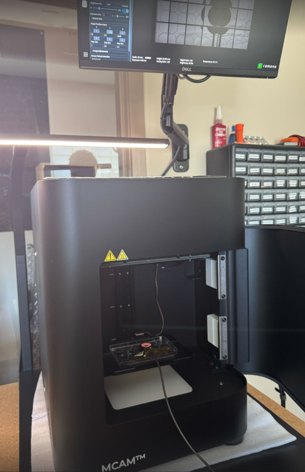
In the following setup, we used a Thorlabs PM100A power meter with a S120C sensor to measure the power at the z-stage location where a wellplate would be in behavior experiments. The sample setup is shown in the image below.
We then increased the intensity of the light source in 10% increments and recorded the measured peak power for 1s pulses.
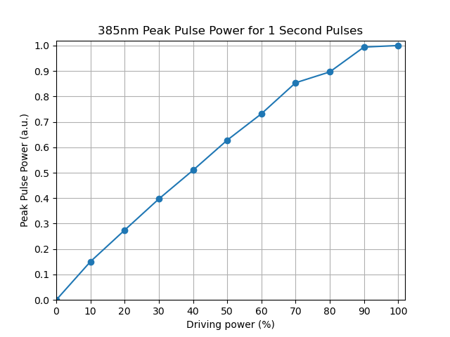
As one can see, the power increases linearly with the intensity saturating roughly at 90%.
Note that while the S120C’s responsivity is not specifically calibrated for 385 nm, the weak response of the photodiode can still be used to estimate the linearity of the flash stimulus.